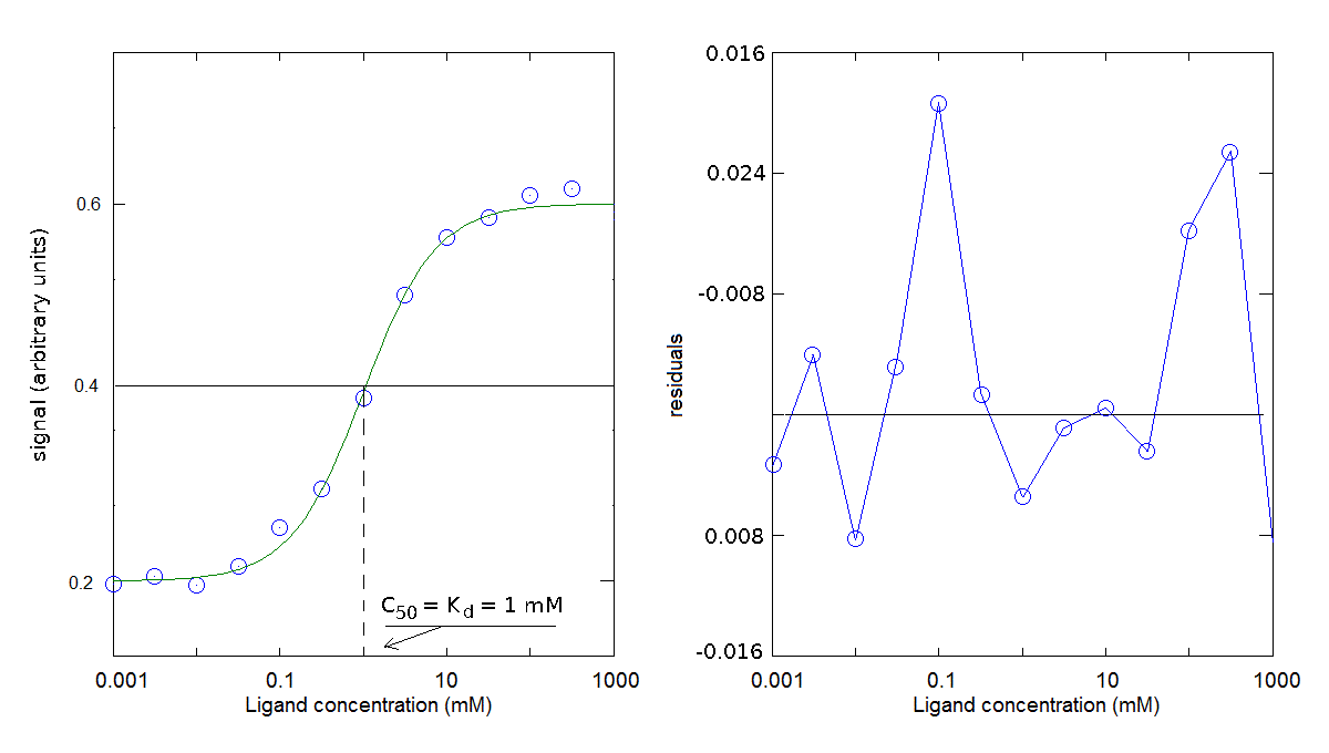
LIGAND BINDING - TUTORIAL #1 answer 1:1 - least squares fit of the signal       Congratulations! This is the statistically soundest procedure to follow.       Unfortunately it is not the easiest to implement. What you have to do is: 1) write down an equation that calculates the signal change as a function of ligand concentration; this must necessarily pass through the ligand binding function but is not limited to it. You use the following equation to calculate the fraction of liganded sites: Y = [PX] / [P]tot = [X] / (Kd + [X]) where Kd is the dissociation equilibrium constant. The signal results: signal = Y x signalPX + (1-Y) x signalP where signalPX is the signal associated to PX at concentration [P]tot and signalP is the signal associated to P at concentration [P]tot. The above equation may be rearranged to: signal = offset + Y x Δ signal where offset is the signal associated to [P]tot in the absence o the ligand (i.e. the lower asymptote of the signal versus log[X] plot), and Δ signal is the difference between the signal associated to [P]tot in the presence of excess ligand and the offset (i.e. the distance between the two asymptote of the signal versus log[X] plot). 2) Use a computer equipped with a non-linear least-squares minimization routine to find the parameters of the above equations (Kd, offset, and Δ signal) that yield the best approximation of the experimental data.       You obtain the following results:       The parameters obtained is Kd = 1 mM (for the dissociation reaction: PX <==> P + X); offset=0.2; Δ signal=0.4.       I remark that the midpoint of the signal change (i.e. the condition [PX] = 1/2 [P]tot) is reached when [X] = Kd. This ligand concentration is called the C50.       Do the residuals look good? 1) Yes 2) No Back one step